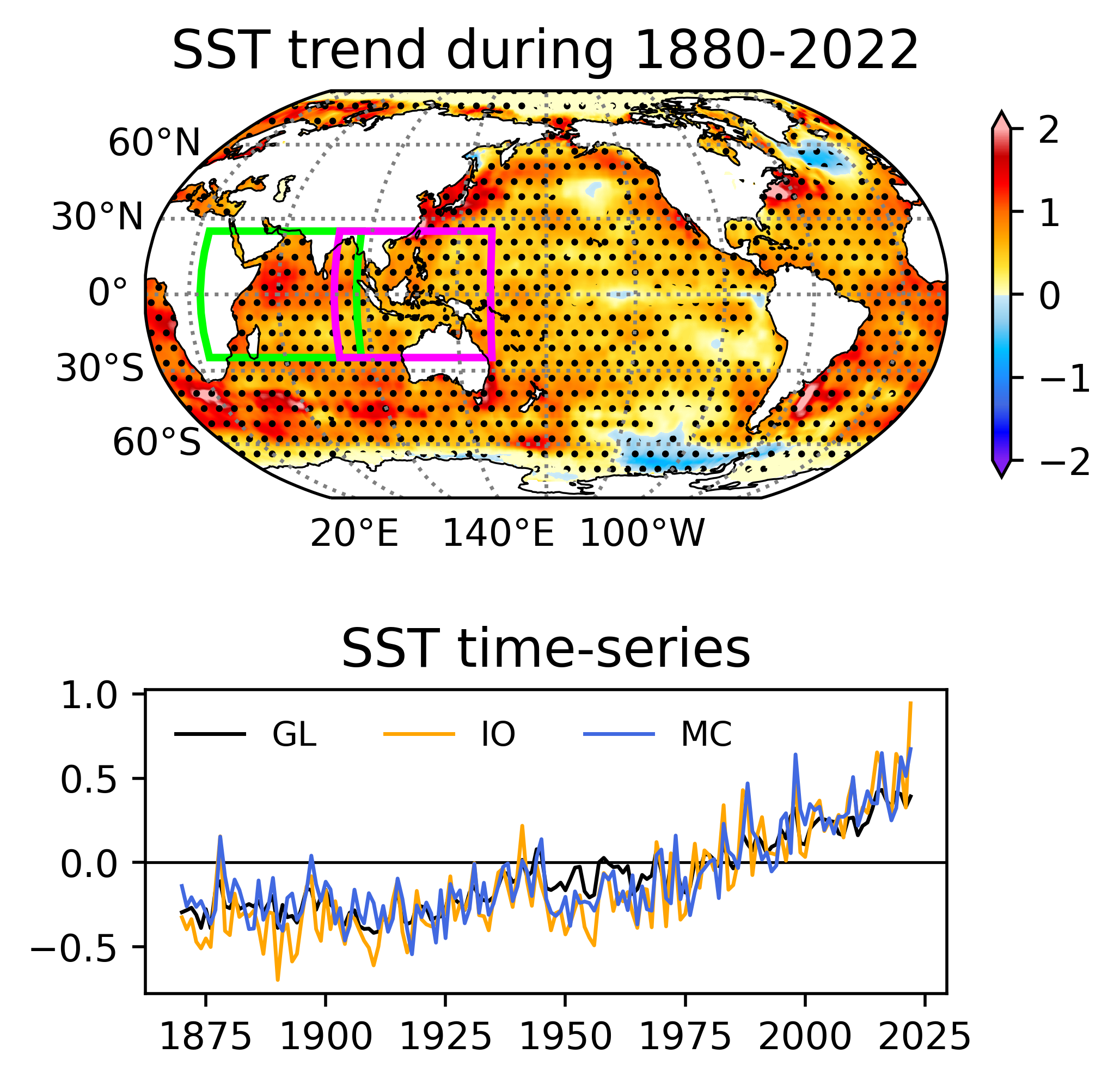
plot: HadISST timeseries long-term trend

Calculate the SST trend and time series

The main figure of this posting

Import python packages

import xarray as xr
import numpy as np
import pandas as pd
import geocat.comp as gc
import cartopy.crs as ccrs
import cartopy.feature as cfeature
import matplotlib.pyplot as plt
from matplotlib.gridspec import GridSpec
from module_mk_trend import mk_trend
import cmaps

from matplotlib.path import Path
import matplotlib.patches as patches

Read HadISST data

# read hadISST data
had = xr.open_dataset('./HadISST_sst.nc')

# rename dimension name
had = had.rename({"longitude":"lon","latitude":"lat"})

# shift longitude from -180~180 deg to 0~360 deg
had = had.assign_coords(lon=(((had.lon+360)%360))).sortby('lon') 

# reverse along lat coordinate from 90~-90 to -90~90
had = had.reindex(lat=list(reversed(had.lat)))

# select SST variable for the specific date_range
sst = had['sst'].sel(time=slice('1850-01-16','2022-06-16'))
sst = sst.where(sst != -1000) # set missing value into nan (_FillValue)

Calculate the SST time series

# calculate anomalies
sst = sst.groupby("time.year").mean('time')
ssta = sst - sst.sel(year=slice(1969,1990)).mean('year')
yrs = (ssta.year[-1] - ssta.year[0] + 1).values # number of years

# select the specific region
ssta_io = ssta.sel(lat=slice(-25,25), lon=slice(25,95))
ssta_mc = ssta.sel(lat=slice(-25,25), lon=slice(85,155))

# weighted average
sst_gl = ssta.weighted(np.cos(np.deg2rad(ssta.lat))).mean(('lon','lat'))
sst_io = ssta_io.weighted(np.cos(np.deg2rad(ssta_io.lat))).mean(('lon','lat'))
sst_mc = ssta_mc.weighted(np.cos(np.deg2rad(ssta_mc.lat))).mean(('lon','lat'))

Calculate the trend and p-value using the Mann-Kendall test

def calc_mk_trend(da):
    trend, prob = mk_trend(da.fillna(-999).values)
    trend = xr.DataArray(trend, dims=da.isel(year=0).dims, 
                         coords=da.isel(year=0).coords)
    trend = trend.where(trend!=-999)
    prob = xr.DataArray(prob, dims=trend.dims, coords=trend.coords)
    prob = prob.where(prob!=-999)
    return(trend, prob)

# get trend and p-value
t, p = calc_mk_trend(ssta)

Plotting the main figure

# plot ...
fig = plt.figure(figsize=(4,4), layout="constrained")

gs = GridSpec(2, 1, figure=fig, height_ratios=[2,1],
        left=0.1, right=0.9, bottom=0.1, top=0.9, wspace=0.05, hspace=0.05)

proj = ccrs.PlateCarree()

axT = fig.add_subplot(gs[0], projection=ccrs.Robinson(central_longitude=180))
#axT = fig.add_subplot(gs[0], projection=ccrs.PlateCarree(central_longitude=180))
axT.set_title("SST trend during 1880-2022", fontsize=14)
axT.coastlines(linewidths=0.5)

cf = axT.contourf(t.lon, t.lat, t*yrs, levels=np.linspace(-2,2,254),
        extend='both', cmap=cmaps.ncl_default, transform=proj)
cbar = fig.colorbar(cf, ax=axT, shrink=0.6, ticks=[-2, -1, 0, 1, 2], pad=0.025)

cs = axT.contourf(t.lon, t.lat, p, colors='none', levels=[0,0.99,1],
        hatches=[None,'...','\\'], transform=proj)

axT.add_patch(patches.PathPatch(Path(verts_IO, codes), edgecolor='lime', facecolor='none', lw=2, transform=proj))
axT.add_patch(patches.PathPatch(Path(verts_MC, codes), edgecolor='magenta', facecolor='none', lw=2, transform=proj))

gl = axT.gridlines(crs=proj, color='gray', xlocs=[20,60,100,140,180,-140,-100,-60,-20],
        ylocs=[-90,-60,-30,0,30,60,90], draw_labels=True, lw=1, ls=':', dms=True)
gl.top_labels = False
gl.right_labels = False

axB = fig.add_subplot(gs[1])

axB.set_title("SST time-series", fontsize=14)
axB.plot(sst_gl.year, sst_gl, c='k', lw=1, label='GL')
axB.plot(sst_io.year, sst_io, c='orange', lw=1, label='IO')
axB.plot(sst_mc.year, sst_mc, c='royalblue', lw=1, label='MC')
axB.legend(frameon=False, ncols=3, prop=dict(size=9))
axB.axhline(0, lw=0.75, c='k', zorder=1)

plt.show()

fig.savefig('python_example_230729_SST_trend_ts.png', dpi=500, bbox_inches='tight')